Contents Previous Next

• Data Structures
  • Types
  • Data keyword
  • Functions
  • Trivial Types
    • Empty
    • Singleton
  • Boolean type
  • Natural numbers
  • Binary Trees
  • Graph
  • List
  • Finite set
  • Indexed sequences or Vectors

Learning a new programming language usually consists of learning two basic things first: 1. Data structures and their APIs 2. Control logic (if/else, loops - for, while, do-while etc)

In a similar fashion, we take a look at how to construct familiar data structures first.

Data Structures

module Lang.dataStructures where

open import Agda.Builtin.Nat public using (Nat)

Types

Agda is an implementation of type theory, a branch of mathematics which deals with Type as an object and various theorems (APIs) for working with Types. A Type presents a notion of an object of a certain kind, i.e. it assigns some extra information to an object.

Programmers might already be well familiar with the notion of Type as it’s use is widespread in programming.

In Type theory, we declare A as a type:

\[ A : Type \]

and say the object x is of type A like:

\[ x : A \]

This, in say scala is done like:

val x:Int = 0

or in C:

int x;

in Agda:

variable
  x : Nat

The Set type is the root of all types, somewhat akin to java’s Object or scala’s Any. Every other Type is a Set, whereas Set itself if of type Set : Set₁. We will look deeper into this at a later stage.

Data keyword

Programming languages often come bundled with some primitive data types like int, float, string etc and some that combine these primitive types into more complex structures, e.g. map or dict (python) can be used to construct say map<string, array<string>> or the Either datatype in haskell, the Option datatype in scala, tuple in python and so on.

Most languages allow creating new data types using either cartesian product or cartesian sum (disjoint union) on a bunch of pre-existing data types and enclosing them inside a container.

Some examples of cartesian product of String, Int and another String would be:

val a : Tuple2[String, Tuple2[Int, String]] = ...

val b : Tuple2[Tuple2[String, Int], String] = ...

val c : Map[String, (Int, String)] = ...

and some example of sums are:

val a : Option[A] = ... // Either A or null

val a : Either[A, B] = ... // Either type A or type B

Some languages also provide the mechanism to define new data types, sometimes by alias-ing a data type with a name like in scala:

type newData = Map[String, List[Float]]

This is called type aliasing.

Others provide the facility to define completely new data types, like haskell does with the data keyword:

-- this states that the type `Bool` can have two values False and True
data Bool = False | True

A haskell datatype can also have constructors. For e.g. if we were to define a shape type which can either be a circle or a rectangle:

data Shape = Circle Float Float Float | Rectangle Float Float Float Float

-- uses the Circle constructor to create an object of type Shape
Circle 1.2 12.1 123.1

-- uses the Rectangle constructor to create an object of type Shape
Rectangle 1.2 12.1 123.1 1234.5

It is important to appreciate that Shape is a new Type, one that did not previously exist before in the language.

The data keyword works in a similar manner in Agda:

-- lets assume the type ℝ, or real numbers is already defined
module _ {ℝ : Set} where
  data Shape : Set where
    Circle : ℝ → ℝ → ℝ → Shape
    Rectangle : ℝ → ℝ → ℝ → ℝ → Shape

Functions

In Type theory, a function f that operates on values of type 𝔸, also called domain of the function and produces values of type 𝔹, also called co-domain of the function, is represented as:

\[ f : 𝔸 → 𝔹 \]

A function in Agda consists of two main parts:

1. Types that the function operates on including:
   1. Domain Type.
   2. Co-domain Type.
2. Clauses − each clause applies to a pattern of argument.

not : Bool → Bool
not true  = false
not false = true

This pattern matching way if typically found in functional programming language and the reader is cautioned that this will be used heavily throughout this work. As Agda is implemented in haskell and its syntax shares high degrees of similarity, it is encouraged to be a bit well versed with basic haskell.

Trivial Types

Empty

An empty type cannot be created cause it has no constructor. This is the most barebones of a data definition.

data ⊥ : Set where

Singleton

A singleton is just a type containing only one object:

data ⊤ : Set where
  singleton : ⊤

The singleton constructor singleton creates a single object of type T.

Boolean type

The boolean type has just two values:

data Bool : Set where
  true : Bool
  false : Bool

Natural numbers

Natural numbers are the integral numbers used for counting, e.g. 0,1,2,3… Natural numbers support an operation called succ for succession, which can be used to create new natural numbers from known ones, e.g. 3 = 2 + 1 = 1 + 1 + 1. Thus, all natural numbers can be created from zero and n successive numbers after zero. All we need to know are:

• zero
• how to increment a given number

and then, increment zero to infinity!

data ℕ : Set where
  zero : ℕ
  succ : ℕ → ℕ

The operations for natural numbers, addition, subtraction, multiplication and powers can be defined as functions in Agda:

_+_ : ℕ → ℕ → ℕ
x + zero = x
x + (succ y) = succ (x + y)

_−_ : ℕ → ℕ → ℕ
zero  − m     = zero
succ n − zero  = succ n
succ n − succ m = n − m

_×_ : ℕ → ℕ → ℕ
x × zero     = zero
x × (succ y) = x + (x × y)

_² : ℕ → ℕ
x ² = x × x

_^_ : ℕ → ℕ → ℕ
x ^ zero = succ zero
x ^ (succ y) = x × (x ^ y)

Examples:

one   = succ zero
two   = succ one
three = succ two
four  = succ three
five  = succ four
six   = succ five
seven = succ six
eight = succ seven
nine  = succ eight
ten   = succ nine

and so on. Here, each member of the integer family can be derived from a smaller member by successively applying succ to it. Such a type is called an Inductive type.

Also note that in the function _+_, we used a new kind of clause:

x + (succ y) = succ (x + y)

Here, we mean that for all inputs of the type x + (succ y) where succ y corresponds to a natural number that has been constructed using a succ i.e. it is (succ y) > 0, return succ (x + y). This pattern is called “pattern matching”. Pattern matching is heavily used all over the functional programming world, e.g. in scala:

(1 to 100).map{
  // pattern match against all values of type integer
  case(y:Int) if y > 5 =>
    y+1
  // if above pattern does not match
  case _ =>
    0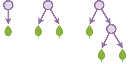
}

Binary Trees

We define a binary tree using the following definition. Note that this merely creates an empty structure of a tree, the nodes or leaves contain no information in them, except for their position in the tree:

data BinTree : Set where
  leaf : BinTree
  node : BinTree → BinTree → BinTree

Now let us augment the binary trees with leaves containing natural numbers in leaf nodes:

data ℕBinTree : Set where
  leaf : ℕ → ℕBinTree
  node : ℕBinTree → ℕBinTree → ℕBinTree

Binary trees with each node and leaf containing a natural number:

data ℕNodeBinTree : Set where
  leaf : ℕ → ℕNodeBinTree
  node : ℕ → ℕNodeBinTree → ℕNodeBinTree → ℕNodeBinTree

Binary trees with each node containing a natural number and each leaf containing a boolean:

data ℕMixedBinTree : Set where
  leaf : Bool → ℕMixedBinTree
  node : ℕ → ℕMixedBinTree → ℕMixedBinTree → ℕMixedBinTree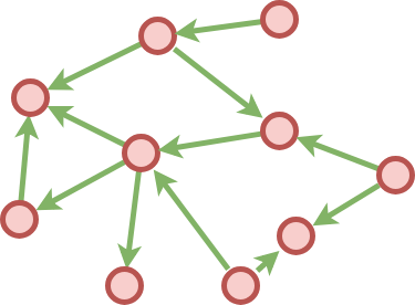

Graph

We define a graph with:

• Vertices containing a natural number
• Edges as triples containing to and from vertices

data Vertex : Set
data Edge   : Set
data Graph  : Set

data Vertex where
  vertex : ℕ → Vertex

data Edge where
  edge : Vertex → Vertex → Edge

data Graph where
  idGraph : Edge → Graph
  _+|+_ : Graph → Edge → Graph

infixl 3 _+|+_

Agda supports “mixfix” operators which combine infix, prefix and postfix operator semantics. Operator arguments are indicated with underscores _. An example would be the infix addition operator _+_ which when applied with two parameters can be written as a + b. Similarly, a prefix operator would be represented as _♠, a postfix one as ♠_. It is also possible to define more complex operators like if_then_else_.

The infixl operator above sets the precedence of the operator +|+.

We can use the above definition to create a graph in the following way:

graph : Graph
graph = idGraph (edge (vertex zero)   (vertex seven))     +|+
                edge  (vertex one)    (vertex three)      +|+
                edge  (vertex seven)  (vertex four)       +|+
                edge  (vertex nine)   (vertex (succ six))

List

A list containing objects of type A can be defined inductively as having:

• An identity element, i.e. an empty list []
• A concat operator which successively creates bigger lists ::

data List (A : Set) : Set where
  [] : List A
  _::_ : A → List A → List A

infixr 5 _::_

and we create instances of lists as:

bunch : List Bool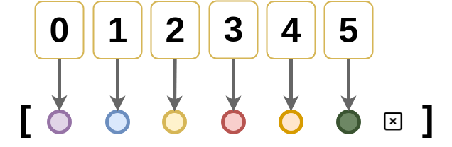
bunch = false :: false :: true :: false :: true :: []

Finite set

A finite set can be considered as a finite bunch of numbered objects, such that each object can be uniquely identified by an integer, thus making the set countable. This count is called the Cardinality of the set.

Formally, a finite set Fin is a set for which there exists a bijection (one-to-one and onto correspondence)

\[f : Fin → [n]\]

where \(n ∈ ℕ\) and [n] is the set of all natural numbers from 0 to n.

This can be represented in Agda as:

data Fin : ℕ → Set where
  id : (n : ℕ) → Fin (succ n)
  succ : (n : ℕ) → Fin n → Fin (succ n)

Fin n represents the set of first n natural numbers, i.e., the set of all numbers smaller than n. We create a finite set of four elements:

fourFin : Fin four
fourFin = succ three (succ two (succ one (id zero)))

For a more in-depth treatment of finite sets, refer Dependently Typed Programming with Finite Sets.

Indexed sequences or Vectors

We now define a finite sized indexed list, also called a vector Vec. The constructor consists of:

• An identity constructor, [] which constructs an empty vector
• A successive constructor cons which inductively builds a vector

data Vec (A : Set) : ℕ → Set where
  [] : Vec A zero
  cons : (n : ℕ) → A → Vec A n → Vec A (succ n)

Examples of vectors :

vec1 : Vec Bool one
vec1 = cons zero true []

vec2 : Vec Bool two
vec2 = cons one false vec1

vec3 : Vec Bool three
vec3 = cons two true vec2

Note that each vector has its size encoded into it’s type. This is not to be confused with set theory based lists, where any two list of different number of elements have the same type.

For example:

val x : List[Int] = List(1,2,3,4,5)
val y : List[Int] = List(1,2,3,4,5,6,7,8,9,0)

both have the same type List[Int].

Another example:

A bool-indexed vector such that only one type can be stored at the same time:

data ⟂ : Set where

data BoolVec(A B : Set) : Bool → Set where
  id₁ : B → BoolVec A B false
  id₂ : A → BoolVec A B true

containsB : BoolVec ⟂ ℕ false
containsB = id₁ three

containsA : BoolVec ℕ ⟂ true
containsA = id₂ four

Functions